P99 Latency: Why the Average Looks Fine and Users Still Retry

The dashboard says average latency is 90 ms. Support says users are refreshing pages, double-submitting forms, and abandoning checkout. Both are true, and the gap between them is where a p99 latency problem lives when the average looks fine. A mean is a sum divided by a count. It cannot tell you whether every request was a little slow or one in a hundred was catastrophically slow, and it cannot tell you that the slow ones are being retried into an even slower state.

The common wrong conclusion is to keep optimizing the median because it is the number on the wall. That makes demos faster and leaves the complaints alone. This post covers how to read a latency histogram, how to tell a queueing tail from a bimodal tail (where some requests do extra work), how a single slow dependency stretches the tail of every caller, and how to confirm a fix by the tail and the timeout rate instead of the mean.

Why the average hides the problem

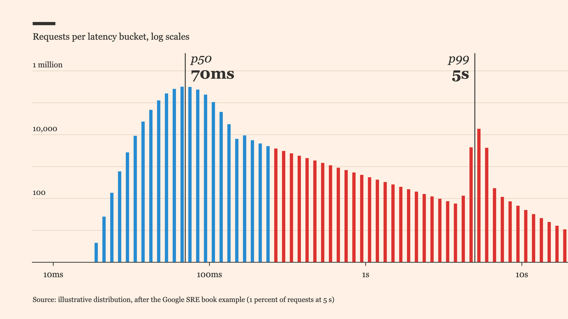
Google's SRE book makes the point with a concrete case: a web service with an average latency of 100 ms at 1,000 requests per second can easily have 1 percent of requests taking 5 seconds (Monitoring Distributed Systems, Google SRE book). The same chapter recommends bucketed histograms over averages and watching the 99th percentile over short windows as an early saturation signal.

Two properties make the tail matter more than its share of traffic suggests:

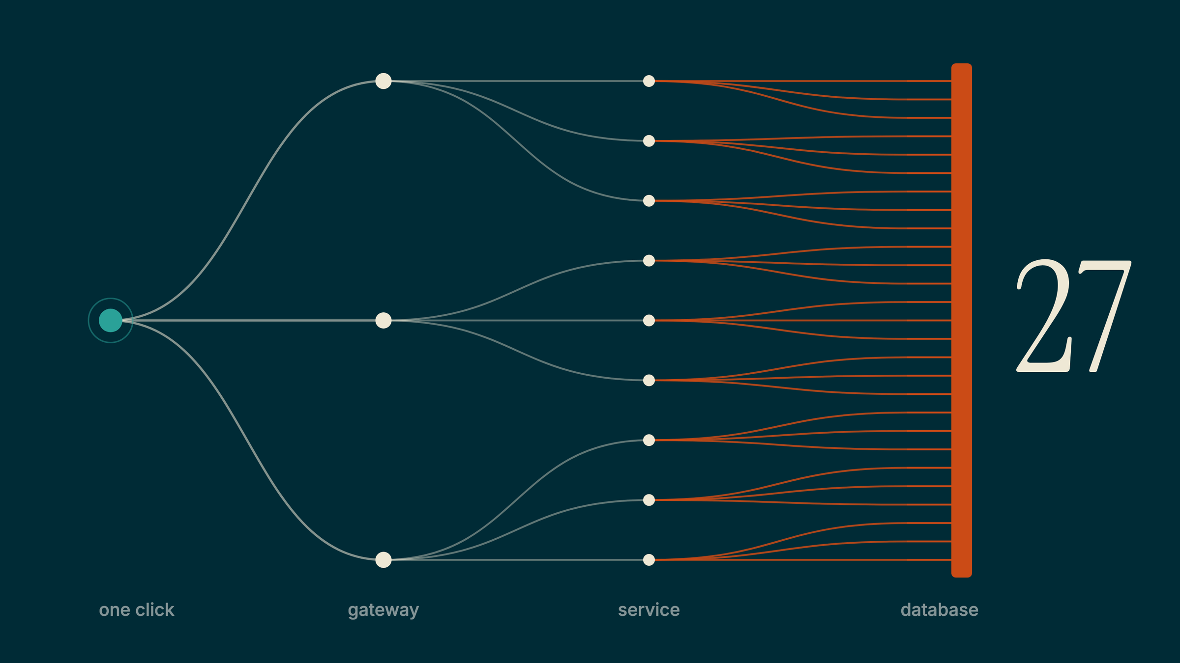
• Users experience it more often than 1 percent. A page that makes several backend calls is as slow as its slowest call. If each call has a 1 percent chance of landing in the tail, a page with 100 independent calls hits at least one slow call about 63 percent of the time (1 minus 0.99 to the 100th power, computed here, not measured). Dean and Barroso's paper "The Tail at Scale" is built on this effect: at warehouse scale, rare slow responses from components dominate what users see (The Tail at Scale, Google Research).
• Slow requests trigger more requests. Clients time out and retry, users refresh, and queues in front of the slow component get longer. The tail feeds itself. See retry storms, backoff, and jitter for the amplification math.

So the question to answer is not "is the p99 number high" but "what are the slow requests doing that the fast ones are not, and is that population large enough to be the reliability problem."

Pick a percentile that matches the complaint

There is no universally right percentile. Match it to the evidence:

• If support tickets describe "it sometimes hangs," look at p99 or p99.9.
• If a timeout on a client is set at 5 seconds and the error rate at the client is 0.5 percent, the percentile that matters is the one that crosses 5 seconds. Compute the fraction of requests slower than that threshold directly instead of guessing at a percentile.
• If a page fans out to many calls, the percentile you need per call is higher than the one you need for the page.

Percentiles also do not average. If each instance exports its own precomputed p99, the mean of those p99s is not the fleet p99. Prometheus documentation states that aggregating precomputed summary quantiles rarely makes sense, and that you should aggregate histogram buckets first and compute the quantile afterward (Histograms and summaries, Prometheus).

Reading a histogram in PromQL

For a classic Prometheus histogram, aggregate buckets across instances, then compute the quantile. The pattern below follows the form in the histogram_quantile documentation:

# p99 per route, aggregated across all instances (illustrative metric name)
histogram_quantile(
  0.99,
  sum by (route, le) (rate(http_server_request_duration_seconds_bucket[5m]))
)

# Fraction of requests slower than the client timeout (5s must be a bucket boundary)
1 - (
  sum by (route) (rate(http_server_request_duration_seconds_bucket{le="5"}[5m]))
  /
  sum by (route) (rate(http_server_request_duration_seconds_count[5m]))
)

Two caveats from the same documentation matter for tail work. First, the function interpolates within a bucket assuming a uniform distribution, so a p99 reported inside a wide bucket is an estimate bounded by the bucket width. Second, when the quantile lands in the highest finite bucket, the function returns that bucket's upper bound rather than infinity. If your top finite bucket is 10 seconds and your p99 is flat at 10 seconds, the real value is at least that, and your buckets are hiding the tail you came to find.

Choose bucket boundaries around the thresholds that matter: the client timeout, the SLO, and the retry deadline. The OpenTelemetry HTTP semantic conventions suggest explicit boundaries for the server duration histogram that run from 5 ms up to 10 seconds (HTTP metrics semantic conventions), which is a reasonable starting point to adjust.

Two tail shapes, two fixes

Once you can see the histogram, the shape tells you which problem you have.

The queueing tail

Every request does the same work, but some wait behind others. The distribution is a single mode that smears to the right as load rises. Signs:

• The tail grows with concurrency or arrival rate, and shrinks when traffic drops.
• Service time inside the handler (measured after dequeue) stays flat while end-to-end time climbs.
• A shared bounded resource, such as a connection pool, thread pool, or lock, shows waiters.

The fix is about capacity and admission, not code speed: raise the bottleneck limit with care, shed or reject load early, shorten critical sections, or add capacity for the peak. For the most common instance, see slow API under load and connection pool wait. The trade-off: capacity sized for a rare peak costs money the rest of the week. Load shedding converts slow successes into fast errors, which is often the right trade but must be a decision, not an accident.

The bimodal tail

A second hump appears. Most requests finish quickly, and a distinct minority takes much longer, at a roughly fixed distance from the first mode. That distance is a clue: it often equals a timeout, a retry interval, a cold cache miss, a slow query for a particular tenant, or a call that only some requests make.

Signs:

• The slow hump is stable across load levels.
• Breaking down by route, tenant, payload size, or cache hit separates the humps.
• Slow requests cluster at suspiciously round values (1 s, 3 s, 5 s, 30 s), which means a timeout or retry timer is shaping the distribution.

The fix is to remove the work only the slow requests do: add the missing index, cache the cold path, move the synchronous remote call out of the request, or stop holding a transaction open across it (see long transactions and external calls).

Telling them apart quickly

1. Plot the histogram (heatmap if you have it), not just a percentile line. One smear versus two humps is usually obvious.
2. Compare p50 against p99 as load changes. If both move together, suspect capacity. If p50 is flat and p99 jumps in steps, suspect extra work or timers.
3. Split the slow population by one dimension at a time and look for the dimension that makes the second hump disappear.

Break the tail down before changing anything

A tail without a breakdown produces guesses. Add dimensions that explain where time went, but keep them bounded. Route templates, a handful of dependency names, and a status class are safe. User ids and raw URLs are not; they belong on traces. The failure mode of unbounded labels is covered in OpenTelemetry metric cardinality and silent overflow.

A useful decomposition for each slow route:

• Queue wait (time between arrival and handler start).
• Handler time split into per-dependency client durations (database, cache, each downstream service).
• Time in retries, recorded separately from the first attempt.

If dependency client histograms exist, compare their tails to the route tail. A route tail that tracks one dependency's tail is that dependency's problem. A fan-out makes this worse: when a route calls many backends and waits for all, the route's median approaches the dependency's tail, which is the effect described in the Tail at Scale paper.

Pull a trace from the slow bucket

Aggregates tell you the tail exists. A trace tells you why. Exemplars connect them: the OpenTelemetry metrics SDK specification describes exemplars as sample measurements that carry the trace and span ids of the active span, so a metrics tool can jump from a histogram bucket to a specific trace (Metrics SDK, exemplars). The default exemplar filter is trace-based, meaning only measurements inside sampled spans are eligible. That has a consequence: if your trace sampling is head-based at a low rate, few slow requests will have exemplars. Prometheus stores exemplars only when enabled and only if the scraped data already carries the trace id (Feature flags, exemplar storage).

To keep the slow ones, tail sampling can retain traces by error or latency, at the cost of a stateful sampler that needs real compute and operation (Sampling, OpenTelemetry). For a small system, a simple alternative is to force-sample any request that exceeds a latency threshold at the handler, so that slow requests always have a trace.

# Illustrative: always keep a trace for requests slower than a threshold.
# Uses the OpenTelemetry Python API; sampler setup is elsewhere.
import time
from opentelemetry import trace

SLOW_THRESHOLD_S = 1.0
tracer = trace.get_tracer("checkout")

def handle(request):
    start = time.monotonic()
    with tracer.start_as_current_span("handle_request") as span:
        try:
            return do_work(request)
        finally:
            elapsed = time.monotonic() - start
            span.set_attribute("app.duration_s", elapsed)
            if elapsed > SLOW_THRESHOLD_S:
                # Mark so a downstream tail-sampling policy can match on it.
                span.set_attribute("app.slow", True)

A collector-side tail-sampling policy can then match on app.slow or on span latency. The trade-off is memory and delay in the collector, because it must hold spans until the trace completes.

When one dependency slows everyone

A single slow dependency stretches the tail of every caller, and the effect is multiplicative with fan-out. Dean and Barroso's mitigations target exactly this: hedged requests (send a duplicate to another replica and take the first answer), tied requests, and micro-partitions that bound how much work a slow node holds. Their abstract notes these techniques reuse fault-tolerance infrastructure and add little overhead (The Tail at Scale).

Hedging is easy to get wrong. Rules of thumb:

• Hedge only idempotent reads, or operations protected by idempotency keys (see idempotency keys and race conditions).
• Delay the second request until the first has been outstanding past a high percentile of normal latency, so most requests never send a duplicate.
• Cap hedges with a budget. Unbounded hedging is a retry storm with better branding.
• Cancel the loser when the protocol allows it.

The less glamorous mitigations come first: per-dependency timeouts shorter than the caller's, bulkheads so one dependency cannot exhaust a shared pool, and a retry policy applied at one layer only.

Timeouts and retries shape the tail you measure

Timeouts and retries do not just react to the tail; they draw it. A request that times out at 5 seconds and retries successfully appears as either an error or a 5-plus-second success, depending on where you measure. That creates the clustered hump at round values described earlier.

Consequences to plan for:

• A tighter timeout shortens the tail and converts slow successes into errors. That can be right (a request nobody is waiting for should not consume capacity), but measure the error rate alongside the percentile or you will mistake failure for improvement.
• Retries multiply load when the system is already slow. If every layer retries, a brief slowdown becomes sustained overload. Retry at one layer, with backoff, jitter, and a budget (retry storms, backoff, and jitter).
• Measure first attempts and retries separately. Otherwise a retry hides the slow first attempt, and the p99 looks better than the experience.
• Record failed and timed-out requests in the latency distribution. The SRE book warns that a slow error is worse than a fast error, and filtering errors out of latency charts can make the service look healthier than it is.

A procedure you can run this week

1. Add or confirm a latency histogram per route with buckets that straddle your client timeout and SLO. Verify the top finite bucket is above the timeout.
2. Chart p50, p99, and the fraction of requests slower than the client timeout, per route, on one panel with request rate.
3. Pick the worst route by slow-request count, not by percentile alone. A 5-second p99 on a route that gets three requests an hour is not your problem.
4. Decide the shape: does the tail move with load (queueing) or stay in a separate hump (extra work)?
5. Break down by one bounded dimension at a time (dependency, cache hit, tenant tier) until a dimension separates the humps.
6. Open exemplar traces from the slow bucket. Confirm that the trace is of a slow request, not a sampled fast one.
7. Make one change and name the prediction in advance: "the second hump disappears" or "pool wait stops growing at peak."
8. Verify by the same panel: the tail percentile, the timeout rate, and the error rate move together in the intended direction, and the p50 may not move at all. If only the mean moved, the fix did not touch the problem users reported.

When not to chase the tail

• Low-volume, internal, or batch endpoints where nobody waits interactively.
• Tails dominated by a rare, known, accepted event, such as a cold start after deploy, where the right action is to exclude or annotate it, not to engineer around it.
• Cases where the cost of capacity or hedging exceeds the cost of the slow requests. Hedging adds load by design, and peak capacity costs money all year.

Optimizing the tail can leave the median untouched and still be the best work available. Optimizing the median when the complaint is a minority of slow requests is the more common mistake.

Checklist

• Histograms with buckets around timeout and SLO, aggregated across instances before computing quantiles.
• A timeout-exceeded rate, not only a percentile.
• Latency of errors and retries included, first attempts distinguished.
• Per-dependency client latency, bounded labels, ids on traces.
• Exemplars or force-sampled traces for slow requests.
• Retries at one layer, with a budget.
• Success judged by tail, timeout rate, and error rate, never by the mean alone.

Sources

• Monitoring Distributed Systems, Google SRE book: average versus tail example, bucketed histograms, p99 as saturation signal, slow errors.
• The Tail at Scale, Google Research: tail dominates at scale, hedged requests, tied requests, micro-partitions.
• Histograms and summaries, Prometheus: aggregate buckets before computing quantiles, error bounded by bucket width.
• histogram_quantile, Prometheus: query form, interpolation, top-bucket behavior.
• Metrics SDK, OpenTelemetry: exemplars carry trace and span ids, trace-based default filter.
• HTTP metrics semantic conventions, OpenTelemetry: suggested duration bucket boundaries.
• Sampling, OpenTelemetry: head versus tail sampling trade-offs.
• Feature flags, Prometheus: exemplar storage requirements.